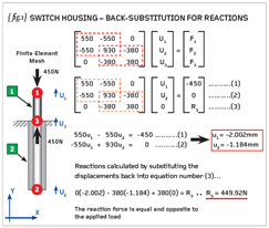
This is the third and final part of a mini-series of articles designed to look into the matrix formulation of the Finite Element Method. After the first two parts we had solved for the primary unknowns – the displacements at node numbers 1 and 2, which were -2.002mm and -1.184mm respectively. {fig.1} shows a repeat of these calculations to save you looking back to the previous article. We can now continue with the rest of the solution.
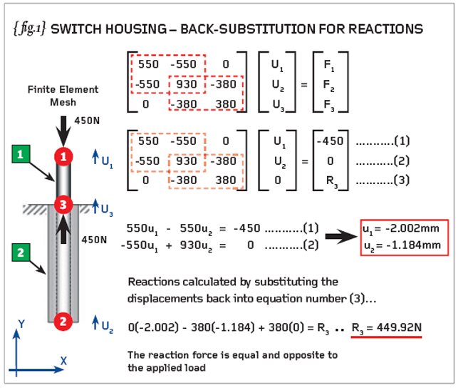
In order to arrive at a unique solution we imposed the boundary condition that the displacement at node number 3 was zero. The corresponding term in the force vector is an unknown “reaction” and this was designated “R3”.
The unknown reaction, R3, can be calculated by substituting the displacements (at nodes 1 and 2) back into equation (3). The reaction becomes +449.92N roughly equal and opposite to the applied load (-450N). In future we need to remember that each time a displacement is constrained to any value (not just zero as shown here) then a corresponding reaction force will be calculated by the FEA.
{fig.1} shows how the element forces can be calculated and here we revert back to the individual element stiffness matrices multiplied by the relevant parts of the displacement solution. Element number [1] is seen to be in a state of compression with a force of 450N applied to each end. Conversely element number [2] is in a state of tension with 450N acting at each end.
{fig.2} also shows how the strains and stresses within the elements are calculated. Here the nominal definition of strain is equal to the change in length (between two nodes) divided by the original length (between those two nodes).

If both elements were pointing in the same direction then the calculation of the nominal strain would be given by the end-node-displacement minus the start-node-displacement, all divided by the original length of the element. [Note: In this model we have “overlapping” elements – one defined in the positive direction and one defined in the negative direction. Therefore we will use a slightly modified method of strain calculation for each].
In the case of element number [1] (negative-Y direction) we define the strain as the start-node-displacement minus the end-node-displacement divided by the original length. In the case of element number [2] (positive-Y direction) we will use end-node-displacement minus start-node-displacement divided by the original length. Refer to the calculations on {fig.2} which render the strains in element [1] and [2] as -0.0134mm/mm and +0.0263mm/mm respectively. The positive sign indicates tension and the minus sign compression.
The element stresses are obtained by multiplying the element strains by the material properties (in this case simply the Young’s Modulus). {fig.2} shows that the stresses for elements [1] and [2] are -5.92MPa and +4.74MPa respectively. The problem is determinate so we know that the applied load of 450N passes through both elements.
Armed with this obvious fact, perform direct stress calculations for the two plastic sleeves and prove to yourself that your hand calculations for axial stress are roughly equal to the Finite Element solution.
That concludes the one-dimensional (line-element) solution of the plastic switch housing problem. If you return to the original definition of the problem you will see that the activation of an internal micro-switch required 2mm of movement under the so-called “failsafe” load of 450N. We achieved a displacement of just over 2mm so our preliminary design doesn’t seem to be too far off track.
{fig.3} shows a two-dimensional section through the switch assembly and we can see this section is repeated for all theta such that we can use an axi-symmetric solution. I have stressed the importance (and accuracy) of such a 2D solution and it is saddening to see that not all CAD-based FEA systems have such a facility! If you can’t perform axi-symmetric analysis with your FEA system then ring the support desk with a loud wake-up call.
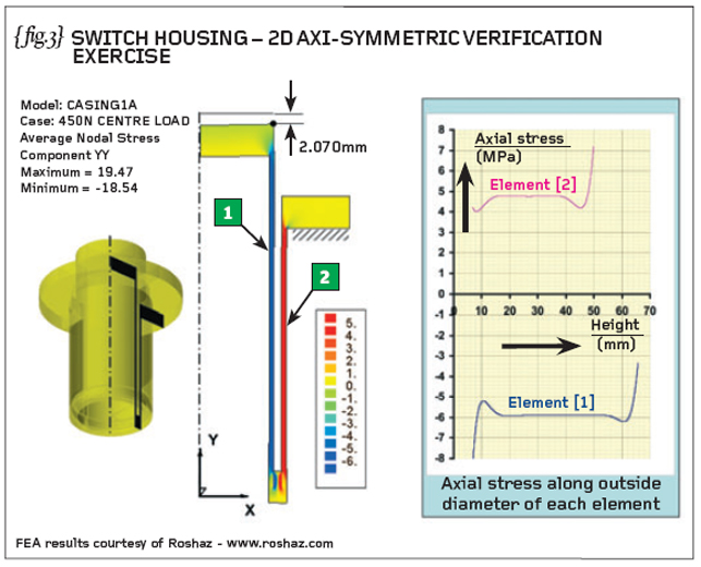
The axi-symmetric analysis, detailed in {fig.3}, represents the two plastic sleeves and the steel collar (perfectly bonded to the plastic sleeves). The applied load was applied to the flat top (6mm thick) by way of normal face pressure and NOT a point load of 450N.
A point load can’t exist in reality so we don’t use it in our simulation. The underside of the collar on the outer sleeve (again 6mm thick) was constrained in the axial direction. The 2D solution gave a displacement of 2.070mm (negative) at the outside diameter of the inner sleeve.
The inset graph shows the axial stress variation along the outside diameter of the two sleeves and, as long as we keep clear of the sudden section changes, then the stresses are very close to those calculated by hand in the one-dimensional solution.
We will look at a new subject next time.
R P Johnson BSc MSc NRA MIMechE CEng
Bob Johnson is technical director of DAMT Limited, a specialist in training courses and consultancy for stress and Finite Element Analysis (FEA).
www.damt.co.uk

Part twelve of an engineering masterclass: Basic Principles of FEA – Part 3