
Welcome to part two of a series of ‘engineering workshop’ articles revising the basics of engineering. The subject for this month’s piece is: forces, moments and free body diagrams. The first thing to address is the difference between mass and force – mass is proportional to the summation of the number of particles in the material that you are considering (i.e. all atomic nuclei – protons plus neutrons) and a force is a “push” or a “pull”.
The important features of mass are (a) it doesn’t want to move when “pushed” (it has “inertia”) and (b) two masses are attracted to each other by an inverse-square-rule relationship. With regard to this second point, Newton identified that the force of attraction was proportional to the product of the two masses divided by the distance of separation squared.
Every day, we experience this force of attraction between the mass of our own bodies and the mass of the earth. Scientists are not really sure why two masses should attract each other, but still!

{fig.1}
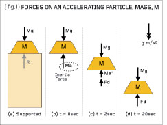
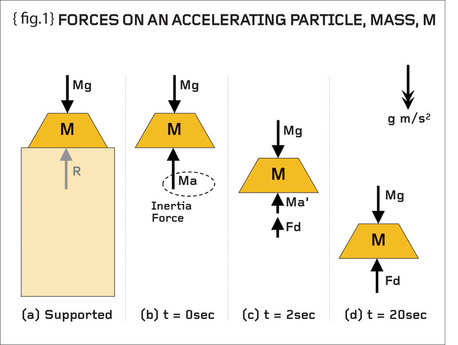
{fig.1} shows a block of steel of mass “M”. If we represent the earth’s “pull” by an acceleration field then we can express the weight force of the mass as “Mg” (mass-times-acceleration). When the block of steel is supported on a concrete plinth (1a) the contact pressure is such that the top surface of the plinth deforms slightly and a reaction force, R, is generated. We therefore have a simple equation in the vertical direction: the reaction force equal to the weight force of the mass (R=Mg). We have shown the mass as a “free-body diagram” – the mass suspended in space with all applicable forces acting on it – it’s as simple as that.
{figs.1b, 1c, 1d} now examine what happens when we remove the support of the plinth – obviously it accelerates towards the centre of the earth until it hits something. At the moment of release (when the mass is still stationary) {fig.1b} we can show the weight force downwards (Mg) and the inertia force (Ma) upwards, where “a” is the acceleration experienced by the mass. [It is important to realise that we can include inertia effects as imaginary forces and treat them like any other force]. Initially, therefore, the acceleration of the particle is equal to the acceleration due to gravity.
After say two seconds {fig.1c} the particle has now gained speed and, because of air resistance, a drag force (Fd) is developed and the acceleration is reduced (to a’). Eventually the particle reaches its terminal velocity {fig.1d} and the downward force, Mg, is matched entirely by the drag force (Fd). Thus we have a set of free-body diagrams that help us understand a simple free-fall. [Note that the buoyancy force of the mass submerged in air has been neglected – this simplification may not be appropriate if submerged in water!].

{Fig.2}
Crank it up
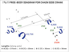
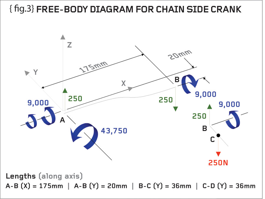
{fig.2} shows the author’s cyclo-cross bike with a pedal force of 250N applied to the chain-side crank while static in the horizontal (3 o’clock) position. Figure 3 shows the corresponding free-body diagram for the crank assuming that there is no rotation (let us assume that the rider has jammed the back brake on). The free-body diagram shows the joggled crank (A-B) and the pedal (B-D) with the load being applied at a point halfway along the pedal (point C).
To represent the loaded pedal as a free-body diagram we must take away its connection to the crank and replace it with the (internal) loads at that joint. It can be seen therefore {fig.3} that the joint must supply a shear force of 250N and a bending moment of 9,000Nmm. If further cuts are made in the pedal then the reader will see that the shear force is constant at 250N between B and C and the moment increases from zero at C to 9,000Nmm at point B in a linear variation.
{Fig.3}
Similarly we can separate the crank arm from the pedal and chainwheel in order to represent the crank as a free-body diagram. Firstly, for equilibrium of the threaded joint at B, we replicate the pedal forces and moments at B, except we reverse the signs and apply these to the pedal end of the crank. We then put the crank into equilibrium by imposing the forces and moments at the bottom bracket bearing (point A). The bottom bracket end of the crank sees a shear force of 250N, a “torsional” moment of 14,000Nmm and the main bending moment of 43,750Nmm. It can be seen that the 20mm joggle in the crank causes the “torsional” (twisting) moment to increase from 9,000Nmm at the pedal end to 14,000Nmm at the bottom bracket end.
If you do a simple check you will see that the pedal (B-D) has no net load in the X, Y or Z directions (force equilibrium). Furthermore there is no net moment about the X, Y or Z directions (moment equilibrium). The same can be seen for the crank (A-B) – there is no net load in the X, Y or Z directions and no net moment about the X, Y or Z directions. Check these – the two components are floating in space under a set of perfectly balanced forces and moments.
More next time when we will attempt to calculate some stresses from the free-body diagrams derived here. In my old days at university the student would get 50% of the mark for a correct free-body diagram so be assured we’ve got it cracked already!
Bob can be contacted at {encode=”bj@damt.co.uk” title=”bj@damt.co.uk”}
Part two of an engineering master class, this month: Forces and moments


